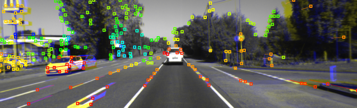
I want to share a plot which took me by surprise. In computer vision, a useful tool for estimating motion is image alignment. Commonly, one may wish to estimate the affine warp matrix which minimizes a measure between pixel values of two images. Below are two aligned images from the KITTI data set, which are demonstrative of forward motion.
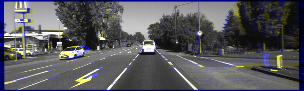
An alternative, which I believe was pioneered by Semi-Direct Visual Odometry, is to align two images by estimating the six parameter transform between the cameras. Usually these are the parameters of the $(\mathfrak{se}(3)$), but could also be three Euler angles plus an $(\langle x, y, z\rangle$) Euclidean transform. Because this method essentially reprojects the first image into the second, the depth field also needs to be known a priori.
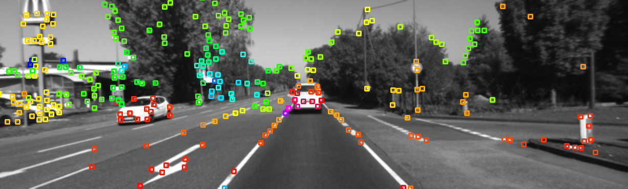
The mathematics involved is surprisingly simple. For a feature based system, several points of known depth will be chosen from the first image $(\mathrm{I}_1$). Around each point, a small rectangular patch $(\mathrm{P}$) of pixels will be extracted and then compared to the second image $(\mathrm{I}_2$) at an offset of $(\langle x, y\rangle$). The goal is for each patch to find an offset which minimizes the below sum.
$$
\begin{equation}
\text{obj}(x, y) = \sum_{i,j}^{\text{patch}} (\mathrm{P}[i, j] - \mathrm{I}_2[i+x, j+y])^2
\end{equation}
$$
Since the objective function is the square of residuals, Gauss-Newton provides a formulation for an iterative update scheme
$$
\begin{equation}
\mathbf{x}^{i+1} = \mathbf{x}^{i} - (\mathbf{J}^T \mathbf{J})^{-1}\mathbf{J}^T\mathbf{r}
\end{equation}
$$
where $(\mathbf{r}$) are the stacked pixel residuals and $(\mathbf{J} = \partial/\partial_{x, y}\mathbf{ r}$). The derivative of a residual,
$$
\begin{equation}
\mathrm{P}[i, j] - \mathrm{I}_2[i+x, j+y]
\end{equation}
$$
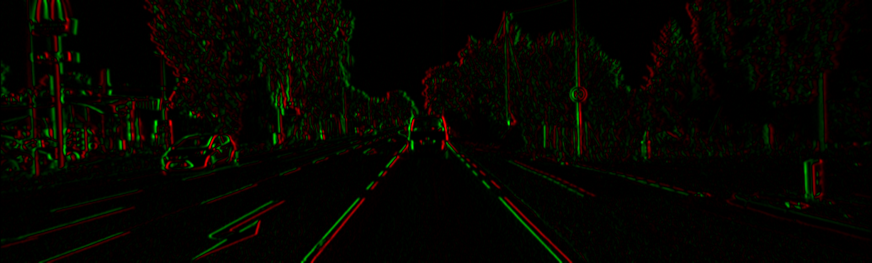
simplifies to the derivative of the only part that depends on $(x, y$), namely $(\partial/\partial_{x, y}\mathrm{ I}_2$). This can be approximated by applying an edge operator, e.g Sobel, to $(\mathrm{I}_2$) in each direction.
$$
\begin{align}
\mathbf{r} =& \begin{pmatrix}
\text{flatten}(\mathrm{P}[i, j] - \mathrm{I}_2[i+x, j+y])
\end{pmatrix}^T \\
\mathbf{J} =& \begin{pmatrix}
-\text{flatten}(\partial/\partial_x \mathrm{ I}_2) \\
-\text{flatten}(\partial/\partial_y \mathrm{ I}_2)
\end{pmatrix}^T
\end{align}
$$
For the sake of completeness, it is worth mentioning that in practice $(\partial/\partial_{x, y}\mathrm{ P}$) is used in place of $(\partial/\partial_{x, y}\mathrm{ I}_2$). Although the maths is technically incorrect, since $(\mathrm{P}$) does not depend on $(x, y$), it turns out that locally during each iteration the role of the patch and the image can be reversed. The trick is to then do the opposite of whatever the Gauss-Newton update step would suggest. The advantages are that $(\partial/\partial_{x, y}\mathrm{ P}$) need only be computed once, and that using a fixed Jacobian seems to make the algorithm more stable.
At any rate, the previous formulation is for a single patch. All patches can be combined into a single iteration as below.
$$
\begin{equation}
\begin{bmatrix}
\mathbf{J}_1 && && && \\
\vdots && && && \\
&& \mathbf{J}_2 && && \\
&& \vdots && && \\
&& && \ddots && \\
&& && \ddots && \\
&& && && \mathbf{J}_n \\
&& && && \vdots
\end{bmatrix}\begin{bmatrix}
\Delta x_1 \\
\Delta y_1 \\
\Delta x_2 \\
\Delta y_2 \\
\vdots \\
\Delta x_n \\
\Delta y_n
\end{bmatrix} = \begin{bmatrix}
\mathbf{r}_1 \\
\vdots \\
\mathbf{r}_2 \\
\vdots \\
\vdots \\
\vdots \\
\mathbf{r}_n \\
\vdots
\end{bmatrix}
\end{equation}
$$
To convert from this form, which individually aligns each patch, to one which globally aligns all patches with respect to a transformation $(\mathbf{T}$), we apply the chain rule.
$$
\begin{equation}
\mathbf{J}_\mathbf{T} = \frac{\partial\mathrm{I}_2}{\partial\mathbf{T}} = \frac{\partial\mathrm{I}_2}{\partial \langle x,y \rangle}\frac{\partial \langle x,y \rangle}{\partial\mathbf{T}}
\end{equation}
$$
Computing this is an exercise in projective geometry, but since our two images are separated predominantly by forward motion, let us further simplify things by instead only computing the image Jacobian with respect to this motion, which we will call $(\mathbf{J}_z$). We now have a function of a single variable, $(\text{ obj}(z)$), which can be plotted.
There is one last implementation detail, which is that the alignment algorithm is performed at multiple image scales. The smoother, lower curves show $(\text{obj}(z)$) plotted at reduced image sizes, where noise is spread across adjacent pixels. The least squares update, as computed using Gauss-Newton, is shown at the bottom.
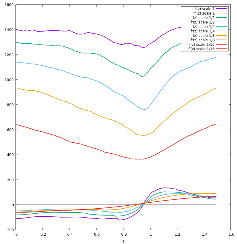
Interestingly, despite multiple local minima, each estimated gradient crosses zero exactly once. This concludes the portion of the blog where I claim to know exactly what's going on.
I believe the key is that $(\mathbf{J}_z$) has been built using only estimates of image gradients, which have all been averaged together to compute $(\partial/\partial_z\text{ obj}(z)$). This has produced a gradient function which has been smoothed in a non-trivial way. The take-away is that this method of estimation seems substantially more robust than numerical differentiation.
It is important to be aware of this phenomena because of how many root finding algorithms work. Some, for example Levenberg-Marquardt, will reject updates which worsen the objective, effectively becoming stuck in a local minimum despite a strong gradient away from the current value of $(z$).
Other algorithms will opt to numerically differentiate with respect to a subset of variables being optimized, even if a method of computing the Jacobian is provided by the user. The rational is that numeric differentiation can be cheaper than computing the full Jacobian, however this post has shown that in some cases, the Jacobian may provide a better estimate of the gradient.
I was unable to get any off-the-shelf least squares solvers to find the correct minimum. I've currently settled for vanilla Gauss-Newton with a termination criterion for when the update direction reverses.